Pivot tables allow you to summarize your data and is available on the following grids:
- Constituents
- Gifts
- Events
- Memberships
- P2P Dashboard
- Volunteer Registrations
- Auctions
- Time Tracking
In the software, pivot tables are used to present summary information, such as cumulative amount received or paid. Since pivot tables are highly customized, they can take some practice to understand and utilize. Pivot tables cannot update the data and the Actions menu is not available from a pivot table. So, you can try different filters, fields, options, and formats to see how the information gets presented without affecting the data itself.
Pivot tables within the software do not have the same functionality of pivot tables available in Excel. If you are an experienced Excel pivot table user, you may wish to just export your data to Excel and create your pivot tables there to utilize all the features available in Excel.
To create a pivot table in the software, begin by adding queries and filters your grid to view the data you would like to analyze further. For example, if you would like to see the summary giving for everyone in a specific date range, begin on the Gifts grid and apply a queries for the date range and types of gifts to analyze.
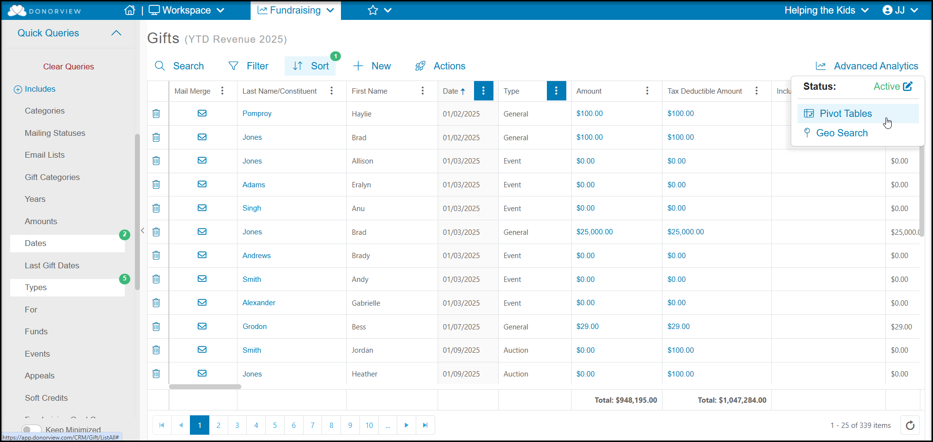
Once your data has been filtered you can create or edit a Pivot Table by clicking the green Advanced Analytics button on the top right of the grid, then Pivot Tables.
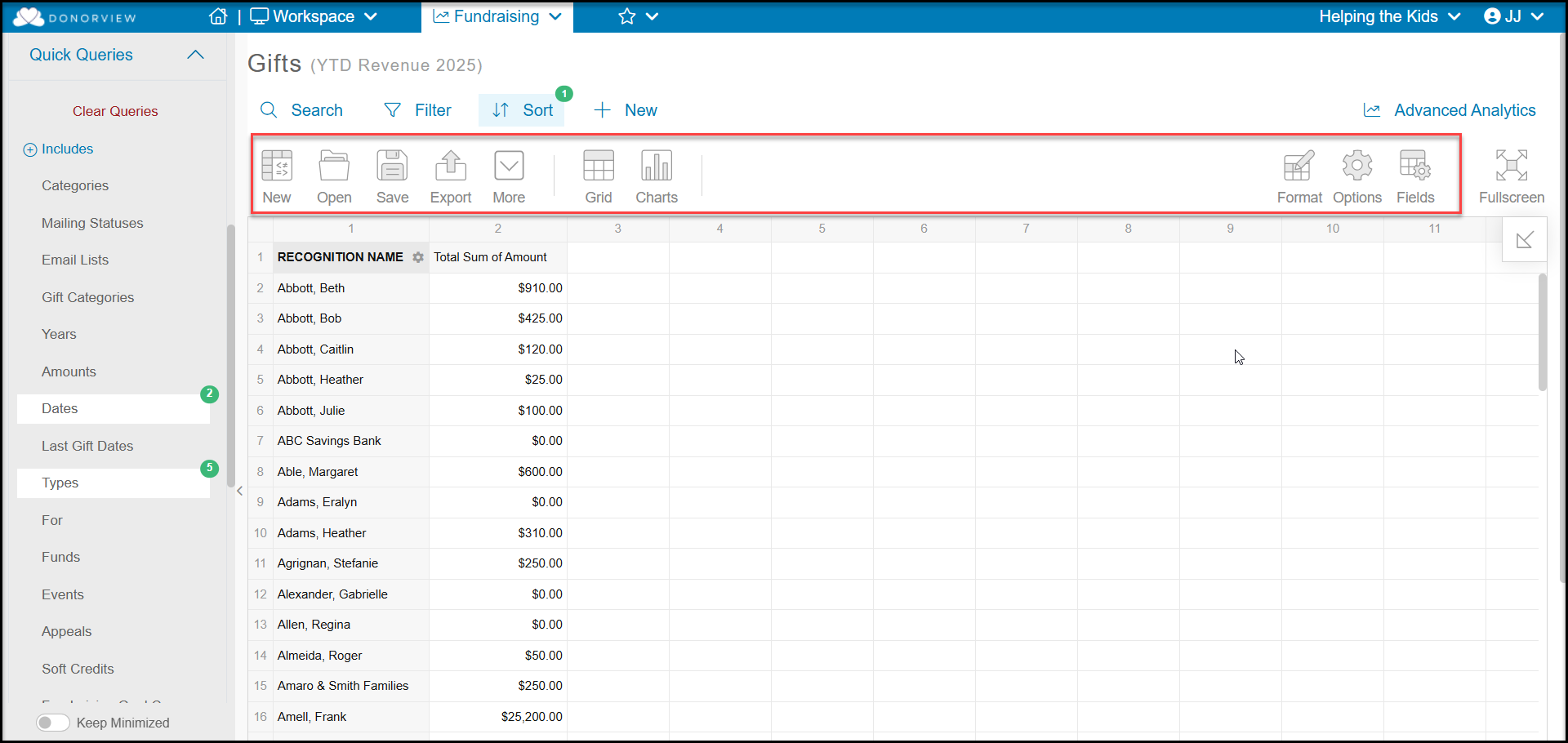
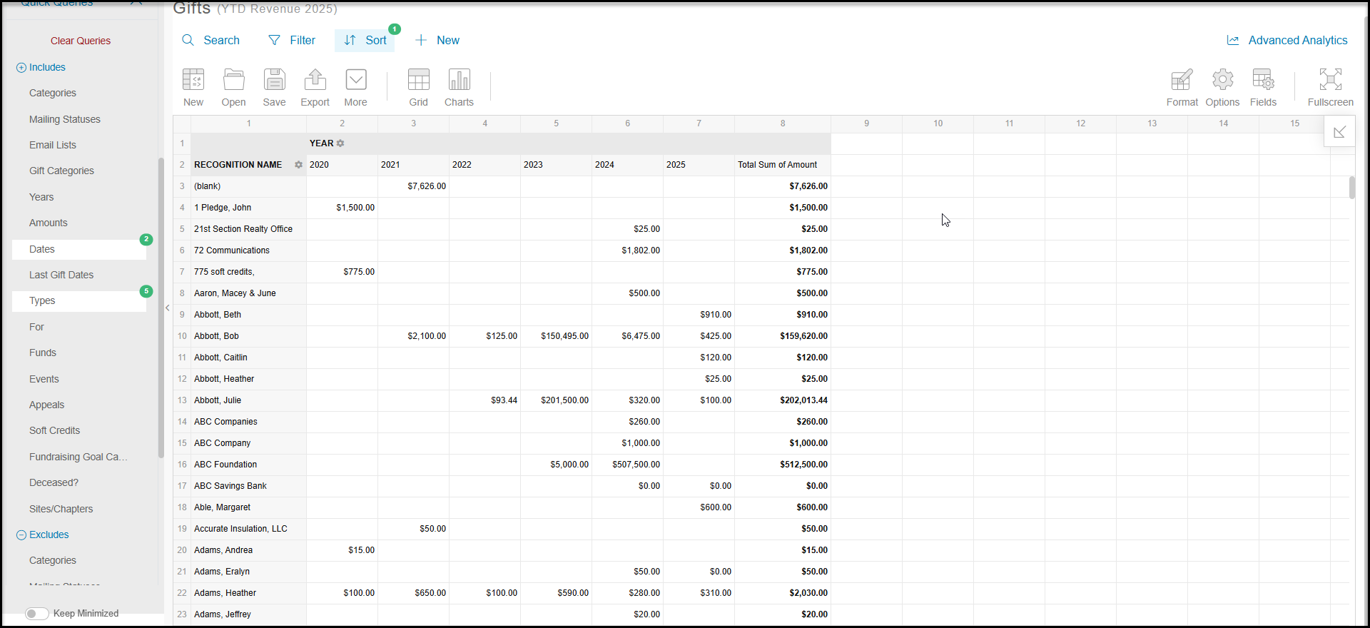
The pivot table starts with a default view showing the cumulative amount received for each constituent in your view.
You can open a saved pivot table using the Open icon and select your previous format to populate the table with the filtered data.
You can start from the default view and build a new table using the Format icon to create new cell formats, the Options icon to modify the layout, and the Fields icon to choose which fields to include in your table.
The default view is shown in a Grid view, but you can switch to a chart view using the Chart icon. You can export the Grid view as an Excel spreadsheet or pdf file using the Export icon. The Chart view can only be exported as a pdf file.
The More icon allows you to rename your table or delete it.
You can start over using the New icon to clear the formats shown and use the Save icon to save your formatted table to use with any data from your grid.
To return to the grid, click Advanced Analytics, then Pivot Tables again.
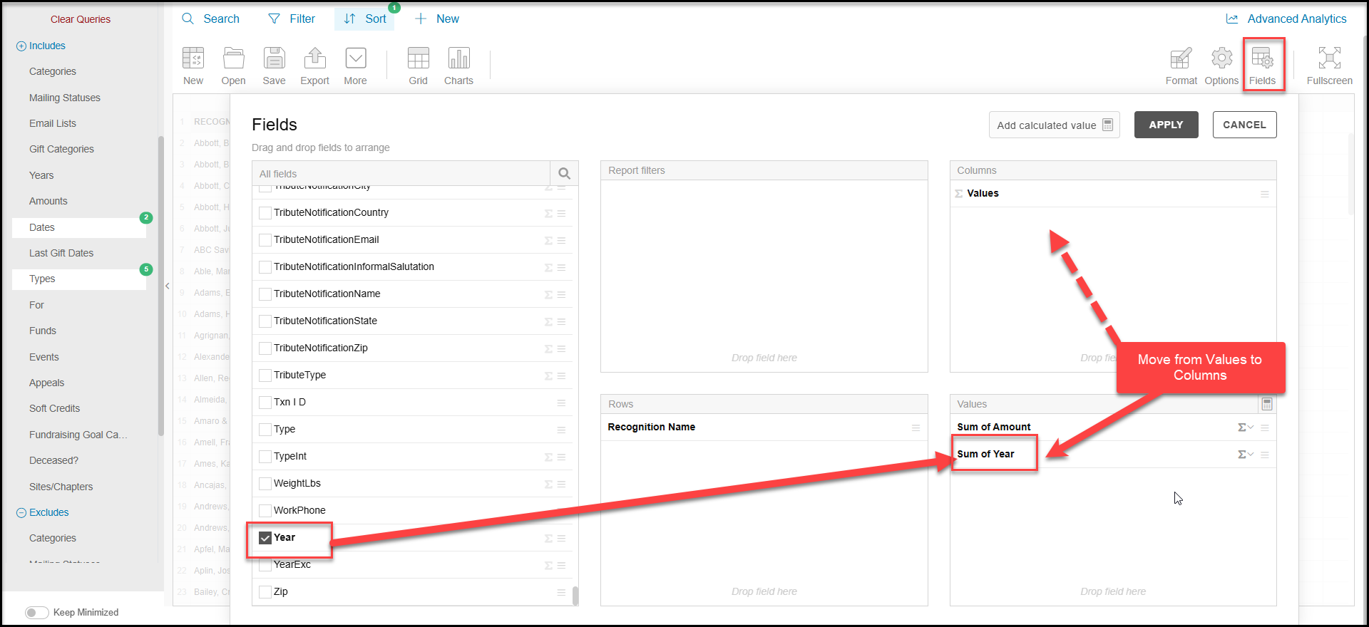
Fields
Fields allows you to add additional columns of data to your pivot table. You can add it as a single summary column by default to the Values area, or if you select a field like “Year,” for example, you can drag it up to the Columns area to have it update your pivot table to show a summary amount for each year.
Click Apply to refresh your pivot table to show the new information.
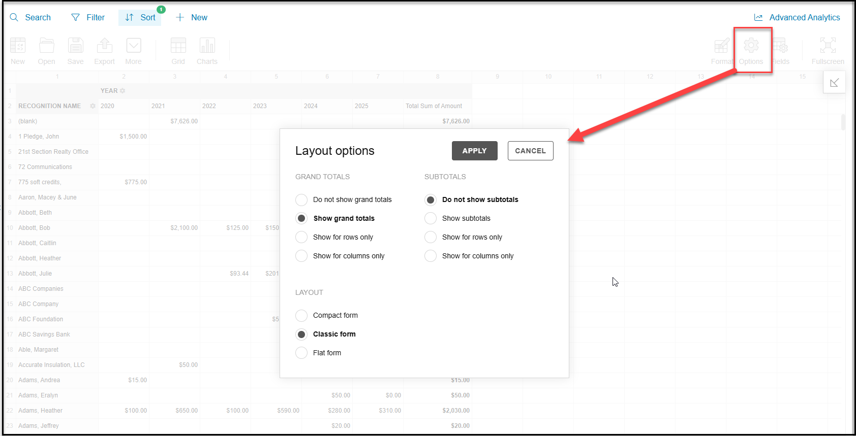
Options
The Options button allows you to update the layout of the pivot table. Choose the Grand Total, Subtotal and Layout options, the click Apply to update the table.
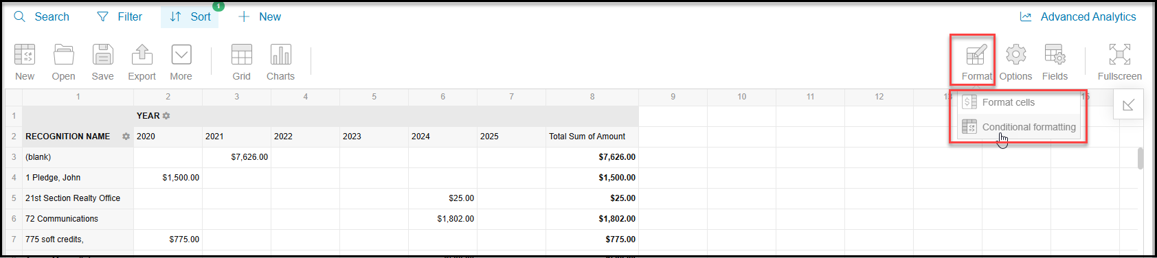
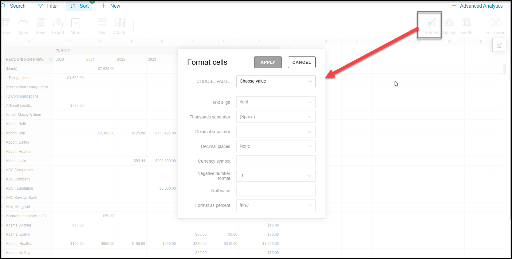
Format
The Format button allows you to format the style of the cells or add conditional formatting to specific values to make them stand out on the table.
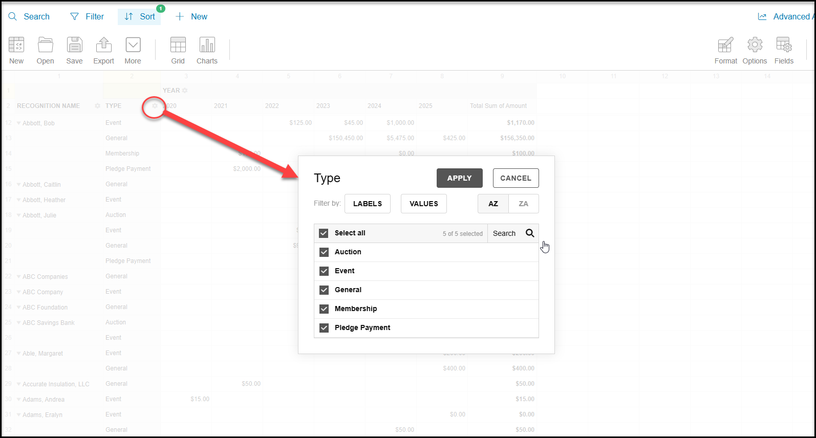
Applying Filters
Filters can be applied to columns when there is a gear icon showing for the columns. If the gear icon is not showing, that information cannot be filter. You would need to export your table to Excel to perform additional filters.
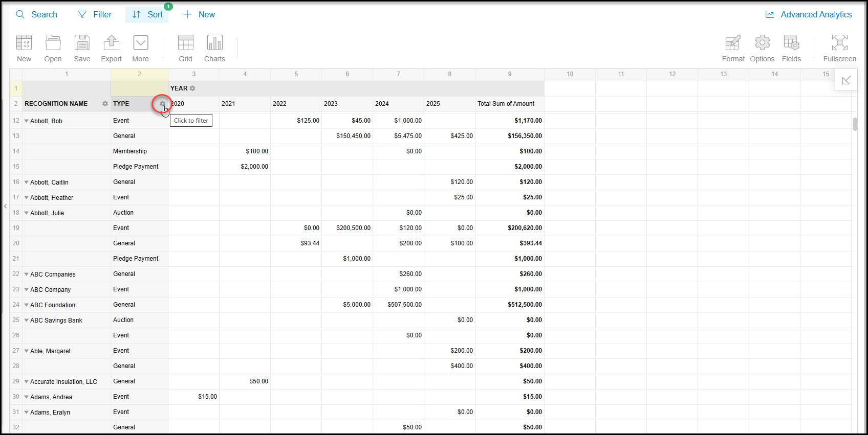
When the gear icon is clicked, a new window will open to allow you to select what to include by labels or by values for numeric fields. Click Apply to update the grid with your selections.